By Luke Roberto, Machine Learning Engineer at Gecko Robotics. As originally published on Notes from the Lab, available on LinkedIn.
Gecko Robotics innovates in robots that Measure and AI that Learns from these measurements in order to derive critical insights about how to best build, operate, and maintain the infrastructure we all rely on. All the data is used to build first-order data layers on our physical world. As a company that increasingly relies on machine learning for our toughest problems, we have a need to innovate and scale our approaches, removing the requirement for tedious labeling processes to train our models. This post will walk you through one of the many interesting ways we are building machine learning systems that will scale beyond our capacity to label all data at Gecko.
Background
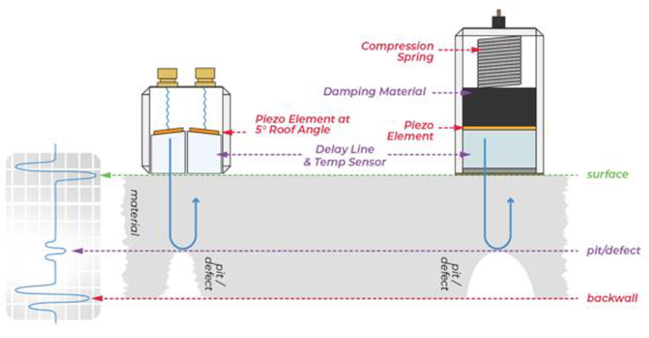
The particular problem we are investigating is that of measuring the thickness of materials nondestructively through ultrasonic testing (UT). Specifically, we look at the problem of Rapid Ultrasonic Gridding (RUG). The robot has an array of ultrasonic transducers that it drags along the surface of an asset and collects data. The transducers on the robot emit an ultrasonic pulse that emanates through the material, reflecting back whenever it meets an abrupt change in material composition (cracks, defects, back wall of the material). This process is depicted in the figure below. These reflections are then measured by the transducer and recorded as a time series. We will refer to these time series as an “A-scan”, which is shown in the second figure below. While this explanation is a simplification, it proves to be a useful mental model for understanding what is happening.
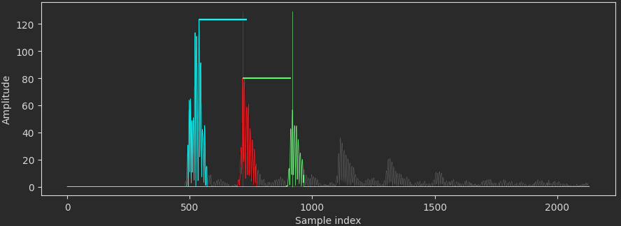
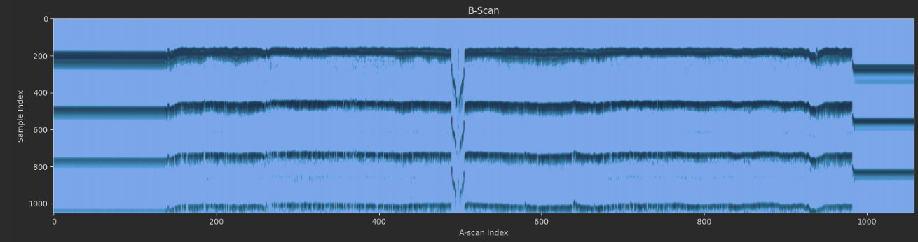
The A-scan represents a single location on an asset and can be used to estimate its thickness and different damage/defect types. Moving the UT sensor across the material and stacking each recorded A-scan can show us how the material is changing across a particular axis. The image below shows a stacked view of these scans and how the thickness of a material may change along a distance. To put a name to a picture, let’s call this a “B-scan”.
In order to build a machine learning model that can begin to automate this process of measuring thicknesses, we would need some source of annotated thickness data for model development, training, and evaluation. Having human data specialists manually annotate individual A-scans is out of the question. However, what if we provided them with tools that allow them to measure larger batches of scans, such as peak finding algorithms and other signal processing tools? This is great! It enables them to annotate a much larger volume of data. An unfortunate side effect is that these algorithms do not adapt; they need to be tweaked from scenario to scenario and require assumptions that could be violated. This can result in a plethora of algorithms that don’t really scale with how diverse the real world is. We would really like to be able to specify the quality of a given measurement so that we could fairly evaluate many different decisions that could be made by a machine learning model, and then guide the model towards measurements that are most aligned with what we deem “correct”.
The task at hand is to then develop learning algorithms that can effectively learn to select these measurement points using the context available to them without the need for human-generated labels.
Reinforcement Learning
Reinforcement learning is a collection of machine learning approaches that are best described as “semi-supervised” learning. Let’s define a few terms first:
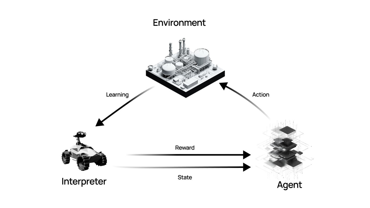
Agent: The model to train. It receives an observation of its environment and will decide to take an action in response. The agent will use the feedback from the environment to update its model of that environment to maximize the quality of its actions in the future.
Policy: A trained agent has a policy, which can be a deterministic or probabilistic function that reads the current observation and returns an action.
Environment: The “world” the agent will interact with. This essentially consumes an action and will transition to some new state.
Reward function: The feedback that the agent receives after it takes an action in the environment. This is typically a single value, but in some cases, it can be a list of different rewards.
Episode: The agent begins in a fixed (or random) state within the environment and then takes a sequence of actions until some terminating state is reached. Learning can happen within or after each episode.
The reinforcement learning agent is then tasked with interacting with the environment, optimizing the actions it takes to improve the reward it receives over time.
Trial And Error
In order to apply reinforcement learning to this problem, we will start simple and work our way up. We need to first define our state space, our action space, and our agent’s reward.
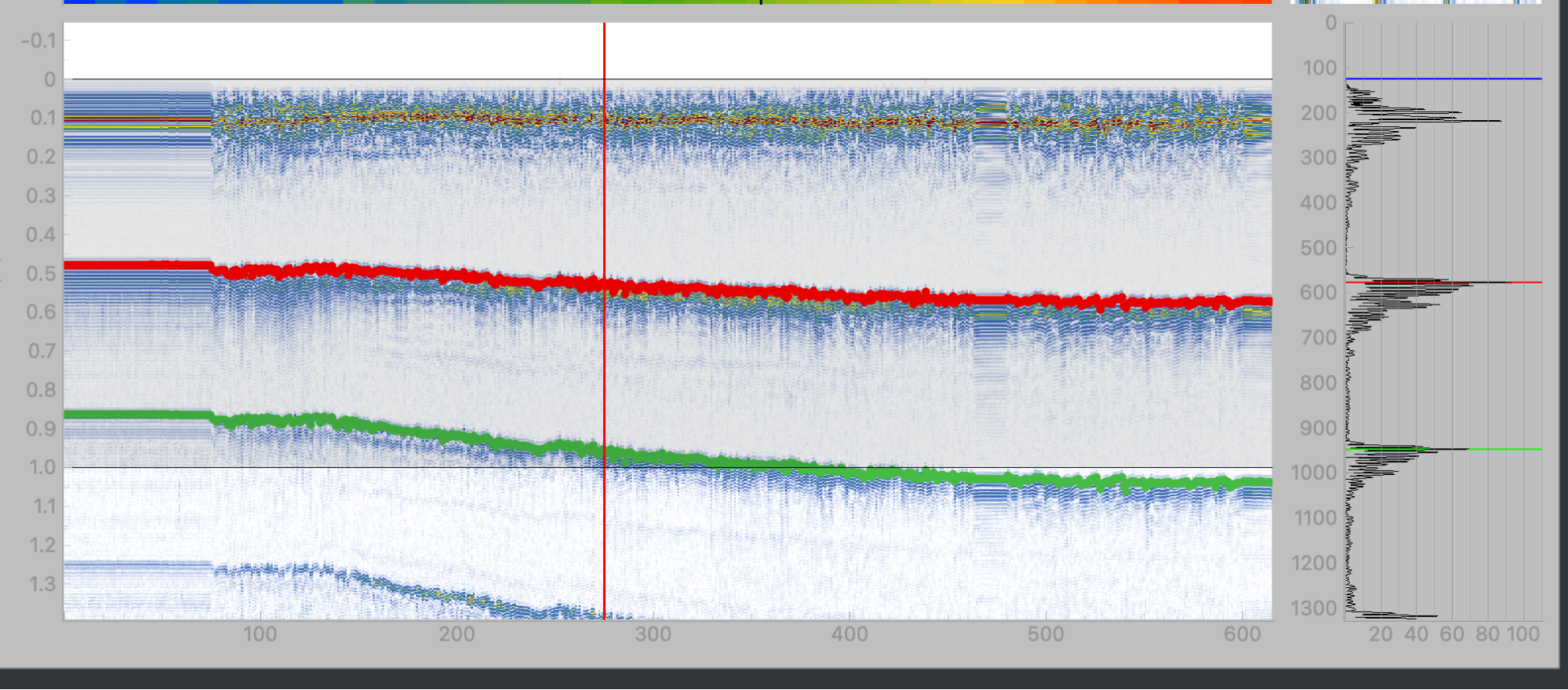
The problem setup will stay simple. We will use our previous B-scan and represent it as an N samples x D distance steps array. Vertical slices of this array represent a single scan, and as you move from left to right, you move in the same direction the robot did when it collected the data. The following photo shows an example of these stacked scans for a run of the robot.
We will use the B-scan to represent the state of our RL agent. For now, we can keep it to something simple, like the index within this run. For the action space, a thickness estimate is essentially a number between 1 and the length of the scan! And finally, to test that our algorithm is working properly, we can try a reward function that is exactly the labels! This is no different than having an agent memorize the correct answer, but it is a building block towards something more complex.
Great! So now we need to push our agent to learn to predict these measurements based on less direct feedback. Note that we are still using the index of the scan as a state, so the agent is not using any features from the scan to make its predictions. This means that it will not generalize to a new run other than this one. This keeps things simple so that we can work on our reward function without the additional complexity of learning a useful feature representation to optimize this reward.
So, what is a good reward? Instead of providing the exact answer, we can provide feedback on how quality the measurement is. What are the elements of a good measurement? Well, one important one is that the thickness replicates across the peaks you can find in a given measurement; in other words, the signal is periodic at the scale of your measurement. If you hop from a peak by the thickness you have estimated and do not land on another peak, then we are breaking the consistency assumption.
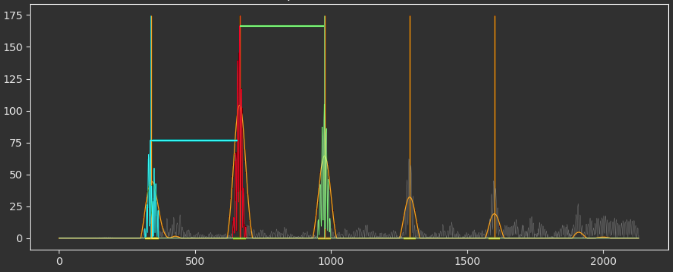
So, you can generate a reward based on this feedback! You can take the thickness predicted by your agent, extract peaks from the signal, and then provide a reward value proportional to the number of peaks that it correctly estimated.
Training an agent on this gets us closer to a more automatic type of supervision that the agent can optimize without human intervention. The other major issue we had not addressed until this point is that of the representation of the observations going into the model. This is where we can turn towards modern Deep Reinforcement Learning methods that are able to parse unstructured data, like full time series. There are a variety of methods in the literature ranging from value network-based approaches—such as Deep Q Networks (DQN), direct policy optimization ones like Proximal Policy Optimization (PPO), or something that combines both as in Stochastic Actor Critic (SAC)—and there are a myriad of other agents in the model zoo. For the purposes of this illustrative example, we trained a simple DQN.
DQNs are in the family of approaches known as “value-based” methods. They learn to build a neural network-based representation of the Q-table, which is a look-up table that tells you the “value” of an action within each state of the environment. This “value” is the sum of rewards the agent gets throughout the episode. Actions that have high value put the agent in a position to accumulate more rewards, so an agent that has trained this model can act greedily with respect to this network to select a sequence of actions that are highly rewarding.
Once trained, we get a model that uses features from the underlying A-scan data and purely from the reward function to infer its thickness estimates. The only information that it receives is the raw signal and feedback based on how its estimates relate to that signal. No need for human supervision to optimize the model policy. Below are the results of the trained model, both on the run it was trained on.
Looking to the Future
In the future, we want to explore a few avenues that could potentially improve the utility and/or performance of this model. A few of these avenues include better reward functions, giving the agent the ability to decide where it should perform a measurement next and providing the agent the ability to refine its previous measurements if it has more context. The reward functions discussed in this post are still limited in the sense that the feedback provided to the agent is heuristic; it is only an approximation of what a quality measurement is. Modifying the reward to reflect more closely what a correct measurement should look like will allow the agent to optimize exactly what is being asked of it.
Another avenue we’re exploring is supporting the agent in attending to non-sequential regions. Our decision to allow the agent to make measurement estimations sequentially was a great start, but you can imagine that allowing the agent to attend to certain regions out of order might allow it establish trends that are specific to this run of the robot (i.e., a long portion of the run might be a single nominal thickness, but a pit causes this to deviate slightly).
Finally, we have limited our exploration to one-shot measurements from the agent. Having the agent attempt to perform the measurements in one shot prevents it from going back to a location with new context from the rest of the measurements it has made. Having the agent update its previous measurements allows it to iterate its decisions until it has settled on a consistent view of what the data represents.
In subsequent posts, we hope to continue this thread of approaches Gecko is developing in order to scale our ability to meaningfully learn from all the data we collect.